 . This will sometimes be written as
  to denote it as the mean of the sample means. The spread of the sampling distribution is called the standard error , the quantification of sampling error, denoted
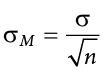
  . The formula for standard error is:
We have come to the final chapter in this unit. We will now take the logic, ideas, and techniques we have developed and put them together to see how we can take a sample of data and use it to make inferences about what’s truly happening in the broader population. This is the final piece of the puzzle that we need to understand in order to have the groundwork necessary for formal hypothesis testing. Though some of the concepts in this chapter seem strange, they are all simple extensions of what we have already learned in previous chapters, especially Chapter 4 and Chapter 5 .
Most of what we have dealt with so far has concerned individual scores grouped into samples, with those samples being drawn from and, hopefully, representative of a population. We saw how we can understand the location of individual scores within a sample’s distribution via z scores, and how we can extend that to understand how likely it is to observe scores higher or lower than an individual score via probability.
Inherent in this work is the notion that an individual score will differ from the mean, which we quantify as a z score. All of the individual scores will differ from the mean in different amounts and different directions, which is natural and expected. We quantify these differences as variance and standard deviation. Measures of spread and the idea of variability in observations is a key principle in inferential statistics. We know that any observation, whether it is a single score, a set of scores, or a particular descriptive statistic will differ from the center of whatever distribution it belongs in.
This is equally true of things outside of statistics and format data collection and analysis. Some days you hear your alarm and wake up easily, but other days you need to hit snooze a few (dozen) times. Some days traffic is light, but other days it is very heavy. Some classes you are able to focus, pay attention, and take good notes, but other days you find yourself zoning out the entire time. Each individual observation is an insight but is not, by itself, the entire story, and it takes an extreme deviation from what we expect for us to think that something strange is going on. Being a little sleepy is normal, but being completely unable to get out of bed might indicate that we are sick. Light traffic is a good thing, but almost no cars on the road might make us think we forgot it is Saturday. Zoning out occasionally is fine, but if we cannot focus at all, we might be in a stats class rather than a fun one.
All of these principles carry forward from scores within samples to samples within populations. Just like an individual score will differ from its mean, an individual sample mean will differ from the true population mean. We encountered this principle in earlier chapters: sampling error. As mentioned way back in Chapter 1 , sampling error is an incredibly important principle. We know ahead of time that if we collect data and compute a sample, the observed value of that sample will be at least slightly off from what we expect it to be based on our supposed population mean; this is natural and expected. However, if our sample mean is extremely different from what we expect based on the population mean, there may be something going on.
To see how we use sampling error, we will learn about a new, theoretical distribution known as the sampling distribution. In the same way that we can gather a lot of individual scores and put them together to form a distribution with a center and spread, if we were to take many samples, all of the same size, and calculate the mean of each of those, we could put those means together to form a distribution. This new distribution is, intuitively, known as the distribution of sample means . It is one example of what we call a sampling distribution , which can be formed from a set of any statistic, such as a mean, a test statistic, or a correlation coefficient (more on the latter two in Unit 2 and Unit 3 ). For our purposes, understanding the distribution of sample means will be enough to see how all other sampling distributions work to enable and inform our inferential analyses, so these two terms will be used interchangeably from here on out. Let’s take a deeper look at some of its characteristics.
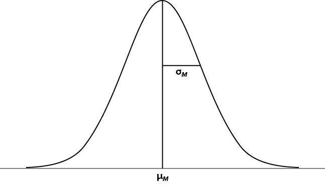
The sampling distribution of sample means can be described by its shape, center, and spread, just like any of the other distributions we have worked with. The shape of our sampling distribution is normal: a bell-shaped curve with a single peak and two tails extending symmetrically in either direction, just like what we saw in previous chapters. The center of the sampling distribution of sample means—which is, itself, the mean or average of the means—is the true population mean, . This will sometimes be written as to denote it as the mean of the sample means. The spread of the sampling distribution is called the standard error , the quantification of sampling error, denoted . The formula for standard error is:
Notice that the sample size is in this equation. As stated above, the sampling distribution refers to samples of a specific size. That is, all sample means must be calculated from samples of the same size n , such as n = 10, n = 30, or n = 100. This sample size refers to how many people or observations are in each individual sample, not how many samples are used to form the sampling distribution. This is because the sampling distribution is a theoretical distribution, not one we will ever actually calculate or observe. Figure 6.1 displays the principles stated here in graphical form.
Figure 6.1. The sampling distribution of sample means. (“ Sampling Distribution of Sample Means ” by Judy Schmitt is licensed under CC BY-NC-SA 4.0 .)
We just learned that the sampling distribution is theoretical: we never actually see it. If that is true, then how can we know it works? How can we use something we don’t see? The answer lies in two very important mathematical facts: the central limit theorem and the law of large numbers. We will not go into the math behind how these statements were derived, but knowing what they are and what they mean is important to understanding why inferential statistics work and how we can draw conclusions about a population based on information gained from a single sample.
The central limit theorem states:
For samples of a single size n , drawn from a population with a given mean and variance s 2 , the sampling distribution of sample means w ill h a ve a m ean  and va r i a nce
 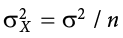 . T h i s di st r i bu t io n will approach normality as n increases.
From this, we are able to find the standard deviation of our sampling distribution, the standard error. As you can see, just like any other standard deviation, the standard error is simply the square root of the variance of the distribution.
The last sentence of the central limit theorem states that the sampling distribution will be more normal as the sample size of the samples used to create it increases. What this means is that bigger samples will create a more normal distribution, so we are better able to use the techniques we developed for normal distributions and probabilities. So how large is large enough? In general, a sampling distribution will be normal if either of two characteristics is true: (1) the population from which the samples are drawn is normally distributed or (2) the sample size is equal to or greater than 30. This second criterion is very important because it enables us to use methods developed for normal distributions even if the true population distribution is skewed.
The law of large numbers simply states that as our sample size increases, the probability that our sample mean is an accurate representation of the true population mean also increases. It is the formal mathematical way to state that larger samples are more accurate.
The law of large numbers is related to the central limit theorem, specifically the formulas for variance and standard error. Notice that the sample size appears in the denominators of those formulas. A larger denominator in any fraction means that the overall value of the fraction gets smaller (i.e., 1/2 = 0.50, 1/3 = 0.33, 1/4 = 0.25, and so on). Thus, larger sample sizes will create smaller standard errors. We already know that standard error is the spread of the sampling distribution and that a smaller spread creates a narrower distribution. Therefore, larger sample sizes create narrower sampling distributions, which increases the probability that a sample mean will be close to the center and decreases the probability that it will be in the tails. This is illustrated in Figure 6.2 and Figure 6.3 .
Figure 6.2. Sampling distributions from the same population with m = 50 and s = 10 but different sample sizes ( N = 10, N = 30, N = 50, N = 100). (“ Sampling Distributions with Different Sample Sizes ” by Judy Schmitt is licensed under CC BY-NC-SA 4.0 .)